An example grid over a beam
[l]
![\includegraphics[scale=0.4]{gridconv.eps}](img836.gif) The aim of the output routine is to simulate what a given telescope would see if it were pointed at
the cloud. The beamsize depends on the diameter of the telescope (
The aim of the output routine is to simulate what a given telescope would see if it were pointed at
the cloud. The beamsize depends on the diameter of the telescope (![]() )
and is given by
)
and is given by
![]() where
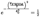
where ![]() is the wavelength of the transition. Since all real telescopes have a non-point like beam it is necessary to simulate the beam.
This is done by placing a grid of points over the beam and calculating the emission at each of those
points. These values are then added together with an appropriate weighting. This is demonstrated in
figure 4.23, where the circle has a radius equal to the beam's FWHM (ie. is two beamwidths in
diameter). The weighting factor for
each position is derived by assuming the beam is Gaussian (ie. follows
is the wavelength of the transition. Since all real telescopes have a non-point like beam it is necessary to simulate the beam.
This is done by placing a grid of points over the beam and calculating the emission at each of those
points. These values are then added together with an appropriate weighting. This is demonstrated in
figure 4.23, where the circle has a radius equal to the beam's FWHM (ie. is two beamwidths in
diameter). The weighting factor for
each position is derived by assuming the beam is Gaussian (ie. follows ![]() ,
where
,
where ![]() is the
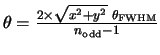
distance from the centre of the beam). Figure 4.24 shows the Gaussian used to model the
beam. The input files give the value for
is the
distance from the centre of the beam). Figure 4.24 shows the Gaussian used to model the
beam. The input files give the value for
![]() (ie. the width of the beam at half the
maximum, for a normalised beam half the maximum is
(ie. the width of the beam at half the
maximum, for a normalised beam half the maximum is
![]() ). However, the beam shape is defined in
terms of
). However, the beam shape is defined in
terms of ![]() (which is the half-width at
(which is the half-width at
![]() of the power) as
of the power) as
The beam model
[r]
![\includegraphics[scale=0.6]{gauss.eps}](img844.gif)
 which can be re-arranged to yield
The unit of each step in the grid (ie. the gap between the dots in
figure 4.23) is given by
![]() where
where
![]() are the number of gridding points to be used (
are the number of gridding points to be used (
![]() must be an odd integer). The
factor of 2 is because the radius of the circle was taken to be equal to the FWHM of the beam,
however,
must be an odd integer). The
factor of 2 is because the radius of the circle was taken to be equal to the FWHM of the beam,
however,
![]() covers the diameter of the circle. So the distance from
the centre of the beam is
covers the diameter of the circle. So the distance from
the centre of the beam is
![]() (where
(where ![]() and
and ![]() are the
are the ![]() and
and ![]() co-ordinates
of the point of interest in say, arcseconds). This can be re-written as
co-ordinates
of the point of interest in say, arcseconds). This can be re-written as
 ,
where the
,
where the ![]() and
and ![]() are the
are the ![]() and
and ![]() co-ordinates of the point of interest but this time in units of
co-ordinates of the point of interest but this time in units of ![]() .
Therefore with the inclusion of the factor 1.665 to convert
.
Therefore with the inclusion of the factor 1.665 to convert
![]() to
to ![]() this
can be substituted into equation 4.53 to give the
weighting for each position as
this
can be substituted into equation 4.53 to give the
weighting for each position as
| (4.54) |
| (4.55) |