Solving the Matrix Equation

In earlier versions of STEN this was done with the NAG routine F04ATF, however, as part of the effort to remove all NAG routines from the program (in order to make it useable on Linux systems for which NAG routines are not available) this has now been replaced by a subroutine called matrix which solves this problem. It does this in several stages. The matrices ${\bf D}$ and $\bf x$ are then considered as a combined augmented matrix and are placed in, first, echelon and then reduced echelon form (where all entries other than the diagonals are zero) by the use of elementary matrix operations (ie. adding a multiple of one line to another does not affect the properties^4.14 of the matrix). This is also often referred to as Gaussian elimination. Each row of the matrix is then multiplied by the reciprocal of the leading term (since the matrix is diagonalised this will be the entry on the diagonal). As this too is an elementary matrix operation it does not affect the properties of the matrix. 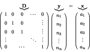These operations have now converted matrix ${\bf D}$ into an $n \times n$ unit matrix and have reduced the associated linear equations to the form

$$\underbrace{\bf D}_{\left( \begin{array}{ccccccc} 1 & 0 & 0 ... ...pace{2mm} \\ a_3 \\ \vdots \\ a_n \\ \end{array} \right)}$$ (4.36)

where the $a_1$, $a_2$, ..., $a_n$ are the numbers generated by the above elementary operations on the $\bf x$ part of the augmented matrix.

It can now be seen that since the ${\bf D}$ part of the matrix equation is a unit matrix the values of $n_1$, $n_2$, ..., $n_n$ and $a_1$, $a_2$, ..., $a_n$ are equivalent, ie. $n_1=a_1$, $n_2=a_2$, ..., $n_n=a_n$ and these are the new level populations for each of the $n$ levels.

Using these level populations the new excitation temperature can be calculated using equation 4.21. This whole procedure is then repeated for each shell. This is then the end of the first iteration as the new excitation temperatures and population levels have now been calculated for each shell throughout the entire cloud. The program then performs a convergence check.