Calculating the level populations

In the program $i$ takes all values for which there are collision coefficients, thus giving $n$ linear equations. However, there are only $n-1$ independent equations here as any one equation will be contained in the other $n-1$. (This can be demonstrated by writing out the two equations generated by allowing only 2 levels, $i=1,2$ and adding them together - they will equal zero and thereby be linearly dependent). Therefore the program replaces one of the equations (the last one - but it could equally well replace any other) with an equation representing the conservation of molecules

$$n_1+n_2+\ldots+n_n=T$$ (4.30)

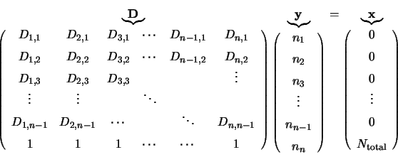
where $T$ is the total number of molecules present. In order to solve this series of linear equations it is necessary to write them as a matrix of the form

$${\bf Dy=x}$$ (4.31)

The subroutine first fills the array elements $D_{i,j}$where $i$ and $j$ take values to cover all levels. The array initially contains just the collision coefficients as it enters the levels subroutine. To each element are then added numbers representing the molecules entering and leaving the level as calculated in the main program:

$$\left(D_{j,i}\right)_{\rm new}=\left(D_{j,i}\right)_{\rm old} +A_{i,j}+\overline{J}_{i,j} \times B_{i,j} \hspace*{5em} j < i$$ (4.32)

$$\left(D_{i,j}\right)_{\rm new}=\left(D_{i,j}\right)_{\rm old}... ...i,j} \times B_{i,j} \times \frac{g_i}{g_j} \hspace*{5em} i < j$$ (4.33)

where $A_{i,j}$ and $B_{i,j}$ are, respectively, the Einstein A and B coefficients and $\overline{J}_{i,j}$ is the radiation intensity at the frequency of the $i \rightarrow j$transition. Note that $\overline{J}$ is represented in the program by the array BPL. Equation 4.32 fills all those array positions which represent downward transitions and equation 4.33 fills all the array positions representing upward transitions. The diagonal elements are then filled using

$$D_{i,i}=-\left(\sum_{j<i}D_{j,i}+\sum_{j>i}D_{i,j}\right)$$ (4.34)

The matrix $\bf x$ in equation 4.31 is filled with zeros except for position $x_n$ (where $n$ is the highest level number) which contains the total number of molecules. This is for the molecular conservation equation (equation 4.30) for which it is also necessary to replace all the $D_{n,j}$ equations with the value one. These $n$ linear equations can now be represented by

$$\underbrace{\bf D}_{\left( \begin{array}{ccccccc} \index{stat... ... \\ 0 \vspace{2mm} \\ N_{\rm total} \\ \end{array} \right)}$$ (4.35)

It can now be seen why the values for the $D_{i,j}$ were set as they were by equations 4.32, 4.33, 4.34. Consider one of the equations given by this array system, say the third one:

$$D_{1,3}n_1+D_{2,3}n_2+D_{3,3}n_3+\cdots+D_{n-1,3}n_{n-1}+D_{n,3}n_n=0$$

The terms $D_{1,3}n_1$ and $D_{2,3}n_2$ represent all molecules leaving level $3$ for lower levels and $D_{4,3}$, $D_{5,3}$, ..., $D_{n,3}$ represent all molecules leaving level $3$ for higher levels. $D_{3,3}$ (which was calculated separately using equation 4.34) represents all molecules entering level $3$ from all other levels. Thus when all these terms are added together the total number of molecules entering and leaving level $3$ should be equal and hence as $D_{3,3}$ is negative the total is zero. Clearly the final line simply sums the number of molecules in each level and sets this equal to the total number of molecules in the system.

The next step is to solve this set of equations (ie. find the values of $n_1$, $n_2$, ..., $n_n$ such that the equations are all true).