Setting up the model cloud

The program starts by reading in all the required data for the cloud to be modelled from the various files. Once this is done it proceeds to construct the model cloud and calculate the parameters necessary for the radiative transfer modelling.

First the sizes of the shells throughout the cloud are calculated using

$$r_{i+1}=r_{\rm min}\left[\left(\frac{r_{\rm cloud}}{r_{\rm min}}\right)^ {\frac{1}{n-1}}\right]^i \hspace*{6em} i=0,\ldots,n-1$$

where $r_{\rm cloud}$ is the cloud radius, $r_{\rm min}$ is the radius of the innermost shell and $n$ is the number of shells.

Next the physical parameters in each shell are worked out (according to the parameters provided in the input files). Once these are known the collision coefficients for each transition can be worked out in each shell. This uses simple linear interpolation of the figures provided for various temperatures in the COEFDATA.DAT file. At present the program can only interpolate for temperatures that lie between the smallest and largest temperatures for which collision coefficients are provided.

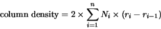
The column density is calculated simply by adding up the individual segments in each shell. Each shell's column density is easily calculated as the density and thickness of the shell is known. The figure returned is

$${\rm column\ density}=2 \times \sum_{i=1}^{n} N_{i} \times \left( r_i - r_{i-1} \right)$$

where $n$ is the number of shells, $N_i$ is the molecular density in the ${\rm i^{th}}$ shell and $r_i$ is the outer radius of the ${\rm i^{th}}$ shell (with $r_0=0$). Note that this is the column density right through the cloud (ie. not just to the centre).