Solving the Radiative Transfer Equation Along a Line of Sight

Although there is no analytical solution to equation 3.13 when $S=f(\tau)$ it is possible to have a computer solve the equation by splitting the integral up into sections

$$I_{\nu_0}=\sum^n_{i=1} \left[ \int^{\tau_{\nu,i}}_{\tau_{\nu,i-1}} S_{\nu,i}(\tau)e^{-\tau_{\nu,i}} d(\tau'_{\nu}) \right]$$ (3.14)

Where $n$ is chosen to be sufficiently large such that over the regions $\tau_{\nu,i-1} - \tau_{\nu,i}$ the value of $S_{\nu,i}(\tau)$ is effectively constant. If this condition holds then it is possible to integrate to give

 

$$I_{\nu_0} = \sum^n_{i=1} \left[ \tau' S_{\nu,i}(\tau)e^{-\tau_{\nu,i}} \right]^{\tau_{\nu,i}}_{\tau_{\nu,i-1}}$$

$$= \sum^n_{i=1} \left[ \left(\tau_i-\tau_{i-1}\right) S_{\nu,i}(\tau)e^{-\tau_{\nu,i}} \right]$$ (3.15)

$$= \sum^n_{i=1} \left[ \tau_{s,i} S_{\nu,i}(\tau)e^{-\tau_{\nu,i}} \right]$$

where $\tau_{s,i}$ is the optical depth of segment $i$ which should also satisfy $\tau_{s,i} \ll 1$. This is now in a format that a computer program can easily handle.

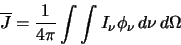
This then is the radiation intensity from one line of sight. In order to calculate the total radiation flux falling on each geometry segment it is necessary to find the average intensity from many lines of sight in many directions. Since the flux will be dependent on frequency it will be necessary to find the flux at several different frequencies and then integrate over frequency to find the total flux.

$$~ \overline{J}=\frac{1}{4\pi}\int\int I_\nu\phi_\nu\,d\nu\,d\Omega \index{flux}$$ (3.16)

Equation 3.16 shows the integral that performs this. $I_\nu$ is the intensity from one line of sight at a particular frequency as given in equation 3.15 (the 0 has been dropped for convenience). $\phi_\nu$ is the function that describes the line profile and for a Gaussian profile is given by

$$\phi_\nu=\kappa e^{-\frac{\nu^2}{\nu_0^2}}$$

This can then be substituted back into equation 3.16 which can be integrated in segments in an analogous manner to equation 3.15 to give

$$\overline{J}=\frac{1}{4\pi}\sum_{d=1}^n\left[\sum_{s=1}^m\le... ...a e^{-\frac{\nu_s^2}{\nu_0^2}}\right)\Delta s \right] \Delta d$$ (3.17)

where $\Delta s$ is the velocity step, $\Delta d$ is the solid angle step size, $n$ is the number of lines of sight (counted by $d$) and $m$ is the number of velocity steps across the line profile (counted by $s$). The solid angle step size is dependent on the number of lines of sight and is simply $\frac{4\pi}{n}$. The line profile function is defined to be normalised so that $\int \phi_\nu \, d\nu=1$. From this it can be deduced that $\kappa=\frac{1}{\sqrt{\pi} \nu_0}$ (this is shown in more detail for a similar calculation next to figure 4.13 on page ). Substituting these into equation 3.17 enables $\overline{J}$ to be written as

$$\overline{J}=\frac{\Delta s}{n\sqrt{\pi}\nu_0}\sum_{d=1}^n\l... ...\nu,s} \index{flux} e^{-\frac{\nu_s^2}{\nu_0^2}}\right)\right]$$ (3.18)

This is the total flux on a particular geometry segment due to the rest of the cloud. This is the information that the statistical equilibrium equations need in order to be able to find the equilibrium population levels that would be caused by such a radiation field.