There are three different processes that cause energy level changes; electronic state changes, molecular
vibration and angular momentum changes. Electronic level changes lead to spectral lines in the UV or visible
regions and vibrational changes lead to spectral lines in the infra red region. However, the spectral lines
of interest in millimetre wave radio astronomy are generally caused by changes in rotation energy levels of
the molecules (ie. angular momentum changes). Most molecules will have either an electric or a magnetic
dipole moment (or both). As the molecule changes its rotation rate (spontaneously or otherwise) the electric
field caused by the dipole moment is changed and a photon is released. The photon carries away the energy
difference between the 2 rotation states. The photon is detected on Earth and many such transitions will
build up a spectral line at frequency
![]() where
where ![]() is the energy difference between the 2
rotation states and
is the energy difference between the 2
rotation states and ![]() is Planck's constant.
is Planck's constant.
Molecules themselves can be divided into several different groups, depending
upon their construction. Which group a particular molecule falls into
depends on the sizes of its principal moments of inertia, designated ![]() ,
,
![]() and
and ![]() and obeying
and obeying
![]() .
The main types of
astrophysical interest are:
.
The main types of
astrophysical interest are:
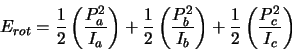
It has already been stated that spectral lines caused by rotation level
changes in a molecule are caused by the loss of rotational energy. Classical
mechanics states that rotational energy is given by
![]() where
where ![]() is the moment of inertia and
is the moment of inertia and ![]() is the angular
velocity.
is the angular
velocity. ![]() and
and ![]() are related by
are related by ![]() where
where ![]() is the
angular momentum. This of course applies to each of the principal axes ie.
is the
angular momentum. This of course applies to each of the principal axes ie.
![]() ,
etc. and so:
,
etc. and so:
| (2.1) |
 |
(2.2) |
Similarly the components of ![]() are given by:
are given by:

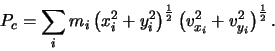 |
(2.4) |
| (2.8) |
| (2.9) |
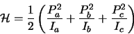
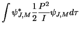
Next consider the Hamiltonian operator, this is related to the classical Hamiltonian
![]() (in 1-D) where
(in 1-D) where ![]() is the momentum and
is the momentum and ![]() is the potential energy.
For a molecule with no external forces acting only the kinetic energy contributes and so:
is the potential energy.
For a molecule with no external forces acting only the kinetic energy contributes and so:
It will now be useful to consider the application of this equation for one molecule in detail.
The simplest possible kind of molecule is one that contains just 2 atoms - ie. a diatomic
linear molecule. From an astrophysical point of view probably the most interesting observable
diatomic molecule is CO and its isotopes . Other molecules such as H![]() would be more interesting but are unfortunately
unobservable as they have no dipole moment.
would be more interesting but are unfortunately
unobservable as they have no dipole moment.
From the definition of a linear molecule ![]() ,
,
![]() ,
,
![]() and so
and so
![]() .
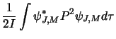
Now using equations 2.7, 2.10 & 2.11
.
Now using equations 2.7, 2.10 & 2.11
| (2.13) |
| (2.14) |
|
|
|
|
|
|
The centre of mass is located on the CO axis
![]() from the O atom.
Using equations 2.3,
from the O atom.
Using equations 2.3, ![]() can next be calculated as
can next be calculated as
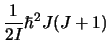
![]() .
This then yields
.
This then yields
![]() which would predict the
which would predict the
![]() transition at
transition at
![]() compared to the measured value of
compared to the measured value of
![]() .
The
slight difference here is due to ignored minor effects, for example, as the molecule
rotates centrifugal effects will cause the bond length to increase slightly, thus
altering the rotation constant.
.
The
slight difference here is due to ignored minor effects, for example, as the molecule
rotates centrifugal effects will cause the bond length to increase slightly, thus
altering the rotation constant.
Unfortunately not all diatomic molecules are as simple as CO. If the molecule has an unbalanced electronic angular momentum this will lead to a splitting of the energy levels due to the coupling of the angular momentum vectors. An unbalanced electronic angular momentum is caused by there being an unpaired electron present. Such molecules have historically been difficult to study as they are generally unstable and therefore short lived on Earth. However, in the interstellar medium several are observable, with CN being one of the prime examples.
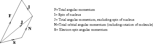
Before continuing it will be instructive to review some notation. Unfortunately this notation is not necessarily consistent with that used in atomic spectroscopy. The total angular momentum of a molecule is made up of several components, namely the angular momentum caused by the rotation of the whole molecule, the orbital angular momentum of the electrons, the electron spin angular momentum and the nucleus spin angular momentum. Each of these is quantised and assigned a quantum number as follows:
In addition the value K occurs in many formulae and is the component of total angular momentum along the principal axis of the molecule.
The vector
![]() ,
which represents the total angular momentum minus the electron spin angular
momentum is made up out of
,
which represents the total angular momentum minus the electron spin angular
momentum is made up out of
![]() and
and
![]() (ie.
(ie.
![]() )
where
)
where
![]() is the vector component of
is the vector component of
![]() directed along the internuclear axis and
directed along the internuclear axis and
![]() is
end over end rotation angular momentum. The component of
is
end over end rotation angular momentum. The component of
![]() (orbital electron
angular momentum) along the internuclear axis is usually given as
(orbital electron
angular momentum) along the internuclear axis is usually given as
![]() .
The values of
.
The values of ![]() are termed the
different electronic states for the molecule and are assigned the letters
are termed the
different electronic states for the molecule and are assigned the letters
![]() for
for
![]() respectively (eg. a
respectively (eg. a ![]() state has
state has ![]() ). To confuse things
even more, for values of
). To confuse things
even more, for values of
![]() the electronic spin angular momentum
interacts with the spin magnetic moment. This necessitates another quantum number to
measure the component of
the electronic spin angular momentum
interacts with the spin magnetic moment. This necessitates another quantum number to
measure the component of
![]() along the internuclear axis - this is denoted
along the internuclear axis - this is denoted
![]() (not the same
(not the same ![]() as for
as for ![]() ! For
! For
![]() is undefined). It takes the values
is undefined). It takes the values
![]() .
The angular momentum along the internuclear axis is then
.
The angular momentum along the internuclear axis is then
![]() .
So
.
So ![]() represents the total angular momentum due to the
electrons for a non-rotating molecule. Note that in the above diagram
represents the total angular momentum due to the
electrons for a non-rotating molecule. Note that in the above diagram
![]() is
only used for molecules in which there is coupling with the nuclear spin, otherwise
is
only used for molecules in which there is coupling with the nuclear spin, otherwise
![]() in which case
in which case
![]() is the quantum number quoted for total angular
momentum. Finally, the nomenclatures are often combined in the format
is the quantum number quoted for total angular
momentum. Finally, the nomenclatures are often combined in the format
![]() where
where ![]() is the multiplicity (eg. for
is the multiplicity (eg. for
![]() are possible) and '
are possible) and '
![]() ' refers to the
letters used to represent the various values of
' refers to the
letters used to represent the various values of ![]() as listed above. Most diatomic
molecules in their lowest state are in the
as listed above. Most diatomic
molecules in their lowest state are in the ![]() state. However, CN in its lowest
state is in the
state. However, CN in its lowest
state is in the ![]() state.
state.
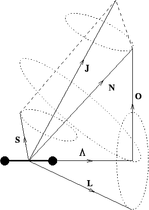
The various angular momentum vectors present in a ![]() molecule can be
represented as in figure 2.2 (from Gordy & Cook [9]). This is referred to as
Hund's case (b). This is an idealised case where the molecule has no orbital momentum
but does possess electronic spin. This causes the spin
molecule can be
represented as in figure 2.2 (from Gordy & Cook [9]). This is referred to as
Hund's case (b). This is an idealised case where the molecule has no orbital momentum
but does possess electronic spin. This causes the spin
![]() to be coupled with
to be coupled with
![]() .
The dotted circles represent the movement of the angular momentum vectors
around a given axis. For example the
.
The dotted circles represent the movement of the angular momentum vectors
around a given axis. For example the
![]() vector precesses about the
internuclear axis and the
vector precesses about the
internuclear axis and the
![]() and
and
![]() vectors both precess about the
vectors both precess about the
![]() axis. Note also that the entire molecule precesses about the
axis. Note also that the entire molecule precesses about the
![]() axis.
axis.
Hund's case (b)
 To calculate the effect that this has on the spectrum of the molecule the Hamiltonian
for the magnetic interaction must be considered. As the field generated by the
rotation of the molecule is proportional to both
To calculate the effect that this has on the spectrum of the molecule the Hamiltonian
for the magnetic interaction must be considered. As the field generated by the
rotation of the molecule is proportional to both
![]() and
and
![]() ,
this
will be given by
,
this
will be given by
| (2.16) |
| (2.17) |
| (2.18) |
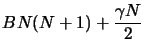 |
(2.19) | ||
| (2.20) |
For some molecules such as CN, however, this is still not the full story. There is the effect of nuclear spin which leads to the hyperfine splitting of the energy levels. Called hyperfine because the splitting generally has an very small effect it is nonetheless an important process that can be very useful in the analysis of molecules such as CN because it splits what would be just one line for a particular transition into several sub-lines of different intensities. Since these sublines have different intensities they also have different optical depths and it is thus possible to gain more information about the structure of a cloud than would be possible if the line were not split.
Since the quantum mechanical description of hyperfine splitting is rather complex it will not be described here.
 Energy levels
 ![\includegraphics[scale=0.8]{transtyp.eps}](img177.gif) Transition types
Transition types